1.
In the domain of the lethal carcinogenic diseases affecting humans, pancreatic cancer is one of the fatal cancers and continues to be a crucial unsolved health problem at the start of the 21st century. Because of the high fatality rates, pancreatic cancer incidence rates are almost equal to mortality rates (22). According to the current health science researchers, this disease causes approximately 30,000 deaths per year in the USA. (1). It is the fourth principal reason for cancer death in the USA and leads to an estimated 227,000 deaths per year worldwide. The incidence and number of deaths caused by pancreatic tumors have been gradually increasing, even as incidence and mortality of other common cancers have been declining. Despite developments in detection and management of pancreatic cancer, only about 4% of patients will live five years after diagnosis, (2). The normal pancreas consists of digestive enzyme-secreting acinar cells, bicarbonate-secreting ductal cells, centroacinar cells that are the geographical transition between acinar and ductal cells, hormone-secreting endocrine islets and relatively inactive stellate cells. The majority of malignant neoplasms of the pancreas are adenocarcinomas. Rare pancreatic neoplasms include neuroendocrine tumors (which can secrete hormones such as insulin or glucagon) and acinar carcinomas (which can release digestive enzymes into the circulation). Particularly, ductal adenocarcinoma is the most frequent kind of malignancy of the pancreas; this tumor (commonly referred to as pancreatic cancer) presents a substantial health problem, with an estimated 367,000 new cases diagnosed worldwide in 2015 and an associated 359,000 deaths in the same year(3)(4). After the detection of pancreatic cancer, doctors usually perform some additional tests to understand better if cancer has been spread or the spreading area of cancer. Different imaging tests, such as a PET scan, can help doctors identify the presence of cancerous growths. With these tests, doctors try to establish cancer's stage. Staging helps explicate how advanced the cancer is. It also assists doctors in deciding the treatment options. The following are the description of the stages used in our dataset according to the definition of the Surveillance, Epidemiology, and End Results (SEER) database. Localized: There is no sign that the cancer has spread outside of the pancreas. 2. Regional: The cancer has spread from the pancreas to nearby structures or lymph nodes.
2. Distant:
The cancer has spread to distant parts of the body such as the lungs, liver or bones.
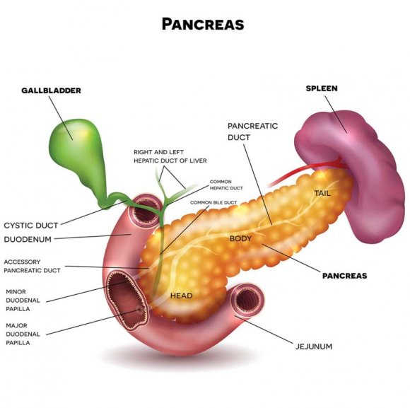
The following Figure 1 shows the different parts of the pancreas.
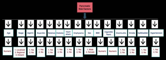
Although, in most cases, pancreatic cancer remains incurable, researchers have focused on how to improve the survival times of patients diagnosed with pancreatic cancer. Cox A schematic diagram of the data used in our study with the description of risk factors is shown in Figure 2, below.
As the above Figure illustrates, we see that twelve out of fifteen risk factors are categorical, having two or more categories. Before we proceed with our main analysis, it is very important to investigate if there is any statistically significant difference between the survival times of male and female patients diagnosed with pancreatic cancer. If any significant differences are found, separate analyses for each gender should be performed. To answer this question, we used the non-parametric Wilcoxon rank-sum test with continuity correction and obtained a p-value of .47, indicating that there is not enough sample evidence to reject the following null hypothesis (H 0 ) at a 5% level of significance. H 0 : There is no statistically significant difference between the survival times of male and female patients. Thus we proceeded with our analysis and modeling by combining the male and female data together to constitute our sample size.
The Cox PH model, proposed by Sir David Cox, is a statistical method that can be used for survivaltime (time-to-event) outcomes on one or more risk factors and their interactions. In survival analysis, the Cox model has been widely recommended for semi-parametric modeling of the survival time relationship as a function of the risk factors. Kleinbaum & Klein (10) gives a good introductory review of the background and methodology, and more detailed descriptions have been provided by Kalbeisch , and Prentice (11) (12). In this section, we give a brief review of the Cox proportional hazards model. An important aspect of the Cox PH model is the hazard function h(t). It measures the rate of the event of occurrence (death) as a function of time t. We define the hazard function as follows; Let random variable T denotes the survival time with cumulative density function F T (t), given by where f (t) = dF T (t) dt is the probability density function (pdf) of the random variable T . The survival function at time t is defined as:
F T (t) = P (T ? t) = t 0 f (t)dt ,S(t) = P (T ? t) = 1 ? F T (t) = ? t f (t)dt .(1)S(t) gives the probability that a specific individual would survive beyond time t. Since S(t) is a probability, 0 ? S(t) ? 1 and S(0) = 1, for T ? 0 from (1) we have,
f (t) = dF T (t) dt = ? dS(t) dt .(2)For continuous survival data, the hazard function plays a very important role. It aims to quantify the instantaneous risks that an event will occur at time t. It is defined as the follows:
h(t) = lim ?t?0 P {t ? T < t + ?t | T ? t} ?t = lim ?t?0 P {t ? T < t + ?t} ?t 1 S(t) = f (t) S(t) .(3)Combining ( 2) and (3), we obtain,
h(t) = ? d dt log{S(t)} .(4)Integrating both sides of equation ( 4) gives an expression for the survival function S(t) in terms of the hazard function h(t). That is,
S(t) = exp ? t 0 h(u)du .(5)Now, from (3) and ( 5) we can express the pdf f (t) as a function of S(t) and h(t) given by,
f (t) = h(t)exp ? t 0 h(u)du .(6)From (3) the cumulative hazard function H(t) can be expressed as:
H(t) = t 0 h(u)du = ?lnS(t) .(7)Now, suppose X i = (X i1 , X i1 , . . . , X ip ) are the realized values of the risk factor for the i th subject.
Then, the Cox PH model (not including time-dependent risk factors or non-proportional hazards) can be expressed in term of the hazard as:
h i (t) = ? 0 (t)exp p j=1 ? j X ij + j =k ? jk X ij X ik , j, k = 1, 2, . . . , p.(8)In the above expression, ? 0 is called the baseline hazard which can be thought of as the hazard function for an individual for which all value of the risk factors are 0. ? j measures the impact of X ij on h i (t). ? jk is the interaction coefficient between j th and k th risk factor of the i th individual and Statistical Data Analysis and Survival Modeling measures the impact of X ij X ik on h i (t). From ( 8), it is clear that the individual hazard is a function of the risk factors and their interactions and is connected through baseline hazard. From (8), we can write,
ln h i (t) h k (t) = p j=1 ? j X ij + j =k ? jk X ij X ik , j = k (9)From the above expression we see that the ratio of log hazard of the i th and k th individual is constant over time. Thus, the name proportional in the Cox PH model. We interpret the hazard ratio (HR) in the following ways:
1. HR = 1; implies that there is no hazard effect. Thus, the risk factors have no relationship with the event probability, thus, no influence on the length of survival.
2. HR > 1 (i.e. equivalently ? i > 0), implies an increase in hazard. That is, the risk factors have a positive association with the event probability, thus, a negative association with the length of survival (bad prognostic factor).
3. HR < 1 (i.e. equivalently ? i < 0), implies a decrease in hazard. That is, the risk factors are negatively associated with the probability of the event, thus, positively associated with the length of survival (good prognostic factor).
A detailed description of the hazard ratio have been provided in ( 14) (15).
We now proceed to develop our most parsimonious statistical model using Cox PH. We initially started by fitting the Cox-PH model to the survival times t as a function of all fifteen risk factors given in Figure 2 together with their two-way interactions. So, there were fifteen risk factors and
15 2= 105 two-way interaction terms. We used a stepwise model selection procedure to select the best model with the minimum Akaike information criterion (AIC = 2ln(L) + 2k, where L is the value of the maximum likelihood function of the model and k represents the number of estimated model parameters) (13). AIC gives an estimation of the relative amount of information missing in the model; hence, the smaller the AIC value, the better the quality of the model. It also deals with the risk associated with overfitting or under-fitting the model. One of the most important assumptions of the Cox PH is proportionality. Initially, all of the risk factors and two-way interactions except age satisfied the assumption. The range of the variable age was [50-90). So, we divided the range into two categories, say [50,70), and [70,90). Now, we use stratification on the variable age. Stratification is one of the tools used by researchers when one of the risk factors does not satisfy the proportionality assumption. The stratification will produce hazard ratios for all other risk factors in the presence of two hazards intrinsic to the level of age. Since age violated the proportional hazards assumption, stratifying it will help meet the PH assumption and provide more valid estimates for all other risk factors. The stratified model allows the baseline hazard ? 0 (t) to vary between strata but controls the effect of the risk factors to be the same for each stratum. For each subject in strata s, s = 1, 2, we have from (8),
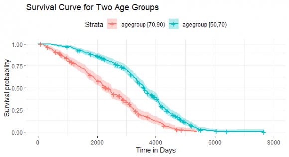
h i (t) = ? 0s (t)exp p j=1 ? j X ij + j =k ? jk X ij X ik , j, k = 1, 2, . . . , p. (s = 1, 2)(10)However, it is not possible to get an estimate of the risk factor (age) separately after stratification. The following Figure 3 illustrates the survival curve for the two age groups. The following Table 1 illustrates the count of each category of all the risk factors after stratification.
The step-wise procedure produced seven out of fourteen significant risk factors and ten two-way interaction terms. There were some risk factors that did not contribute to the hazard individually, but, interacting with other risk factors, their effect was significant. Thus, we added those risk factors in our proposed model. That is why there are thirteen individual risk factors and ten interactions in the model (11). In the following model (11), we denote "Y" to indicate yes of a specific answer of a risk factor. That is, the specific category possesses the characteristic. For example, to answer the question "does the patient ever have diabetes?" the individual answers "yes." To describe any particular category of the risk factor stage, we use L, R, and D which are the first letters of Localized, Regional, and Distant. To describe male and female category of the variable Sex, we use the letters M and F, respectively. The most parsimonious model that we found after removing the insignificant (p-value > 0.05) term from the model is given as follows:
ln h i (t) ? 0 (t) = ? ? ? ? ? ? ? ? ? ? ? ? ? ? ? ? ? ? ? ? ? ? ? ? ? ? ? ? ? ? ? 0.3X 2R + .5X 2D ? .53X 3Y +.61X 4Y ? .37X 15Y + .87X 6Y ?.6X 5Y ? .7X 8Y ?.35X 9F + .0037X 11 ? .51X 12Y + .15X 13Y +.28X 14Y ? .56X 4Y X 13Y + .41X 3Y X 9F +.6X 3Y X 15Y + .01X 2R X 11 + .68X 12Y X 9F +.32X 15Y X 9F ? .47X 15Y X 14Y ?.52X 2R X 4Y + 2.18X 2R X 8Y + .8X 15Y X 12Y(11)Thus, the proposed statistical model consists of thirteen individual risk factors and ten interactions that contributes to the hazard.
The above equation ( 10) can be written as:
h i (t; X ij , X ij X ik ) = h 0s (t)exp p j=1 ?j X ij + j =k ?jk X ij X ik , j = k(12)We can express the Cox-PH model (11) in the form of the survival function, S(t), by employing equation ( 5) from Section 3. Thus, the survival function the model can be expressed as;
?i (t; X ij , X ij X ik ) = exp ? t 0 h i (t; X ij , X ij X ik )dt = exp ? t 0 h 0s (t)exp p j=1 ?j X ij + j =k ?jk X ij X ik dt = exp exp p j=1 ?j X ij + j =k ?jk X ij X ik ? t 0 h 0s (t)dt = exp ? t 0 h 0s (t)dt p j=1 ?j X ij + j =k ? jk X ij X ik = S 0s (t) p j=1 ?j X ij + j =k ? jk X ij X ik(13)where ?is (t; X ij , X ij X ik ) is the survival function at time t for i th individual and s th , (s = 1, 2) stratum. S 0s (t) is the baseline survivor function for each stratum s = 1, 2. After the estimation of ? and ?jk by partial likelihood (16), S 0s (t) can be estimated by a non-parametric maximum likelihood method (17). The co-efficient estimates of parameters ? and ?jk are given in the third column of Table 2.
Table 2 below displays the estimates of the model coefficients/parameters, their hazard ratios (HR) (exp( ?)), standard error of coefficients, statistical significance, and 95% confidence interval. We proceed to rank the significant contributing risk factors and their significant interactions based on the prognostic effect on the survival times of patients diagnosed with pancreatic cancer using the hazard ratio (HR). Thus, we rank from the most contributing risk factor to the least contributing risk factor to pancreatic cancer patient's death or survival times.
The above Table 2 describes different information, including the hazard ratio of all seven significant risk factors and all ten significant interactions used in the model. A positive estimated coefficient/weight ( ? > 0) implies higher hazard rate, and thus a bad prognostic factor. on the contrary , a negative estimated coefficient/weight ( ? < 0) implies a lower hazard rate, and thus a good prognostic factor. For example, ? 9F = ?0.35 from Table 2, implies females are good prognostic of the survival time of pancreatic cancer; thus, females have a lower risk of death (higher survival rates) of cancer than males. The exp( ?) is the hazard ratio (HR). Thus, exp(?0.35) = .7 < 1 for gender female means being a female has a reduced risk of dying with pancreatic cancer than being a male. The ranking of the significant risk factors from Table 2, based on the HR, shows that the interaction between cancer stage (Regional) and patient having Emphysema (X 2R X 8Y ) is the highest prognostic factor to the survival of pancreatic cancer, followed by patients having diabetes (X 6Y ), and Relatives who have pancreatic cancer (X 5Y ) is the least prognostic factor. We also provide the 95% confidence interval of the hazard ratios (HR) corresponding to the risk factors; that is,
P [U CL ? HR ? LCL] ? 95%where U CL and LCL are the upper and lower confidence limits and we are at least 95% confident that the hazard ratios will fall into the limits. The following Table 3 provides the three popular global tests of significance which our model is based on. As, the following table shows, our proposed model (11) is highly significant based on all the three statistical tests. Assumptions of Cox ph Model and Validation of the Proposed Model
In order to apply the CPH model, we must verify that the following three key assumptions are satisfied, prior to its implementation. Failure to satisfy these assumptions will bring about inaccurate decisions about the subject matter. The data consists of times T 1 , T 2 , . . . , T n which are either observed survival times or censored times with censoring indicators ? 1 , ? 2 , . . . , ? n . ? i = 1 implies T i is observed, and ? i = 0 implies T i is censored. Suppose there are p fixed covariates/risk factors Z 1 , Z 2 , . . . , Z n and R i be the risk set at time T i denoted as R i = {j : T j ? T i }. Given the setup, the partial likelihood, proposed by Cox (1975) is defined by:
L(?) = n i=1 ? i ? T Z i ? log j?R i exp(? T Z j ) .(14)Let ? be the usual estimator of ? that minimizes L(?) in (13). Also, let t (i) be the i th ordered observed survival time and Z (i) and R i the corresponding covariate vector and risk set. Then SCHOENFELD'S RESIDUALS are defined as follows:
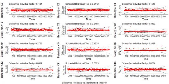
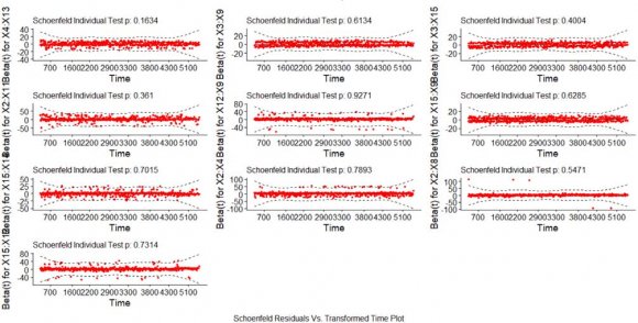
ri = Z (i) ? j?R i Z j exp( ?T Z j ) j?R i exp( ?T Z j ) .(15)The following Figures 5 and 6 illustrate the plot of the scaled Shoenfeld residual against time for all risk factors and interaction terms used in the model (11), respectively. It shows that there is no pattern as a function of time. Thus, the residuals are randomly scattered with no systematic departures from the horizontal fitted smoothing spline deep line (that is, the residuals are independent of times). A formal test for the PH assumption is given in Table 4. The covariates and the global test are non-statistically significant given by the large p-values. This is a further justification of the validity of the PH assumption for our proposed model. We have included all fourteen risk factors and ten interaction terms in the table. The number of terms in
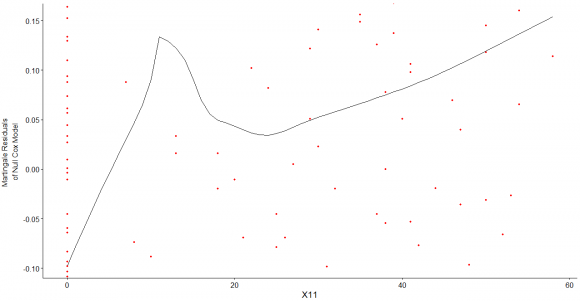
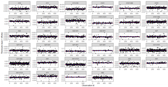
Mi = ? i ? Î?"0 (t i )exp p j=1 ?j X ij + j =k ?jk X ij X ik , j = k. ,where ? i denotes the event indicator for i th observation, Î?"0 (t i ) is the estimated cumulative hazard at the final follow-up time for the i th observation. Martingale residuals, M i , have a skewed distribution. We have, Mi = 1 for for maximum possible values and Mi = ?? 3. Testing influential observations and Outliers: Often influential observations can cause problems with modeling results. In order to check the influential observations, we visualized the dfbeta values. The dfbeta values estimates the of the i th -patient observation on the regression coefficients ? j . A high value of dfbeta must be investigated carefully. Another method for checking influential observations is by assessing the deviance residuals (symmetric/normalized transformation of the Martingale residuals) plot. The deviance residual is defined by
d i = sin( Mi ) ? 2 ? Mi ? ? i log(? i ? Mi ).In the above equation, Mi implies d i = 0. The square root shrinks the large negative martingale residuals, while the logarithm transformation expands those residuals that are close to zero. The distribution of the residuals must approximately be symmetrical around mean zero and standard deviation of one. A very large/small/distant deviance residual values indicate influential observations or outliers. Figure 8 below implies that none of the observations is exceedingly influential individually, on average.
3. Results and Discussions
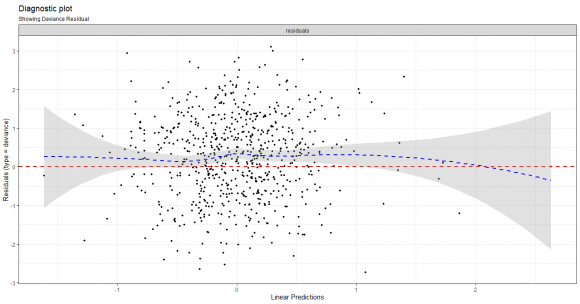
The following Figure 9 plots the deviance residual and the residual pattern looks fairly symmetrical around zero. The mean deviance residual for our model is .2 which is very small.
Given the risk posed by pancreatic cancer in the past few years, it is imperative to investigate the clinical diagnosis and enhance the therapeutic/treatment strategy of pancreatic cancer. The primary treatment for most types of pancreatic cancer is chemotherapy. Sometimes, with chemotherapy, specific therapy drugs are used. Usually, surgery and radiation therapy do not fall under crucial treatments VII.
4. Conclusion
for pancreatic cancer, but they might be used in exceptional circumstances. Also, the treatment approach for children with pancreatic cancer can be slightly different from that used for adults. Several research approaches and statistical methodologies (23) (24) have been developed to cure pancreatic cancer patients and boost their survival times. Chakraborty & Tsokos (to be published) performed data-driven research on pancreatic cancer patients by performing parametric analysis to improve the survival probabilities of patients of different cancer stages. In the present study, we initially investigated if there exists any statistically significant difference between the true mean survival times of the male and female pancreatic cancer patients using the Wilcoxon two-sample rank-sum test. The p-value (.47 > .05) of the test result suggests that there is no evidence of a significant difference between the true mean survival times of the males and the females. Hence, we proceed to perform to develop the Cox-PH (CPH) model with the combined information of male and female patients. While developing the CPH model, it is very important to justify the model assumptions. In the preliminary analysis, we found that all of the risk factors except age (X 1 ) did not satisfy the proportional hazard assumption. Thus, we introduced stratification in our model by dividing the covariate age into two groups. By doing stratification, we obtained more valid estimates of the other covariates, and the proportional hazard assumption was satisfied for all risk factors, including age. Performing stratification, we restrict the effect of the covariates to be the same for each stratum. Our final developed Cox-PH model given by equation ( 11) identified all the significant risk factors along with all the significant interaction terms as contributing to the hazard. After building our model, we proceed to rank all significant individual risk factors and all possible significant interactions according to the hazard ratio, as shown in Table 2. From Table 2, we observe that X 6Y (patients having diabetes), X 4Y (patients taking ibuprofen regularly), X 2D (patients who are in stage distant (Cancer has spread to distant parts of the body)), X 9F (sex), and X 15Y (hypertension) are the most contributing risk factors individually to the survival of patients with a hazard ratio (HR) of 2.39, 1.83, 1.63, .7, and .7, respectively. For the risk factor X 6Y , HR = 2.39 indicates a strong association between the patients having diabetes and increased risk of death due to pancreatic cancer. Keeping the other covariates constant, being a diabetic patient has a 2.39-fold increase in the hazard of death; that is, 2.39-fold increased risk (or decreased survival). It is important to note that according to the American Cancer Society, one of the main risk factors of pancreatic cancer is diabetes which is supported by our study. Also, we have found that those who take ibuprofen regularly have an increased risk of 1.83-fold than those who do not take the medication on a regular basis. Also, being a female has approximately 30% less hazard than a male patient. Among the most significant interactions we have X 2R X 8Y , X 15Y X 12Y , X 12Y X 9F , X 3Y X 15Y , X 3Y X 9F , X 15Y X 9F , and X 2R X 11 with hazard ratio 8.84, 2.28, 1.98, 1.83, 1.5, 1.37, and 1.01 respectively. The most contributing risk factor is an interaction term (X 2R X 8Y ) (patients with emphysema and cancer stage regional with HR = 8.84). However, they do not contribute significantly to survival. We see that X 15Y (hypertension) has a lower risk of survival (HR = .79). However, interacting with X 12Y (diverticulosis), it has a hazard ratio of 2.28. Also, interacting with X 3Y (person who uses Aspirin Regularly), it has a hazard ratio of 2.28. It is also important to note that X 3Y individually has lower risk (better survival) with HR = .6. Although X 12Y (diverticulosis) and X 9F (female) has a hazard ratio less than one, their combined effect remains significant with HR = 1.98.
In this study, we have estimated the survival probabilities of patients diagnosed with pancreatic cancer using the semi-parametric Cox proportional hazard (CPH) model. We believe the proposed Cox-PH model given by equation (11) gives an accurate estimate of the survival probability of patients diagnosed with pancreatic cancer. The stratification of the age produced more reliable estimates of the risk factor included in the CPH model. We identified seven significant risk factors and ten significant interaction terms as contributing to the survival probability of patients diagnosed with pancreatic

| group [70,90). | ||
| Risk Factors | Count | |
| Localized 135 | ||
| Stage | Regional 178 | |
| Distant | 364 | |
| Aspirin | Yes No | 333 344 |
| Ibuprofen | Yes No | 168 509 |
| Relatives | Yes No | 650 27 |
| Diabetes | Yes No | 83 594 |
| Heart attack | Yes No | 84 593 |
| Emphysema | Yes No | 19 658 |
| Sex | Male Female | 388 289 |
| BMI | 677 | |
| Cigarette Years | 677 | |
| Diverticulosis | Yes No | 41 636 |
| Smoke | Yes No | 404 273 |
| Gallbladder | Yes No | 98 579 |
| Hypertension | Yes No | 256 421 |
| Rank Risk Factors coeff( ?) HR [exp( ?)] [S.E( ?)] Lower 95% Upper 95% | |||||||
| 1 | X 2R X 8Y | 2.18 | 8.84 | .96 | 1.32 | 59.1 | |
| 2 | X 6Y | .87 | 2.39 | .33 | 1.2 | 4.6 | |
| 3 | X 15Y X 12Y | .8 | 2.28 | .38 | 1.07 | 4.87 | |
| 4 | X 12Y X 9F | .68 | 1.98 | .39 | .92 | 4.25 | |
| 5 | X 4Y | .61 | 1.834 | .25 | 1.27 | 2.62 | |
| 6 | X 3Y X 15Y | .6 | 1.831 | .18 | 1.11 | 3.02 | |
| 7 | X 2D | .5 | 1.63 | .17 | 1.16 | 2.3 | |
| 8 | X 3Y X 9F | .41 | 1.5 | .18 | 1.06 | 2.13 | |
| 9 | X 15Y X 9F | .32 | 1.37 | .18 | .96 | 1.96 | |
| Volume XXI Issue III Version I | 10 11 12 13 14 15 16 17 | X 2R X 11 X 9F X 15Y X 15Y X 14Y X 13Y X 4Y X 3Y X 2R X 4Y X 5Y | 0.01 -.35 -.37 -.47 -.46 -.53 -.52 -.6 | 1.01 .7 .69 .63 .63 .6 .59 .55 | .007 .13 .16 .26 .2 .13 .3 .2 | .99 .54 .5 .42 .42 .45 .33 .35 | 1.05 .91 .95 .94 .94 .77 1.05 .84 |
| D D D D ) F | |||||||
| ( | |||||||
| Medical Research | |||||||
| Global Journal of | |||||||
| © 2021 Global Journals | |||||||
| Test | Test Statistics Value df p-value | |
| Likelihood Ratio Test | 96.6 | 34 7*10 ?8 |
| Wald Test | 100.8 | 34 2*10 ?8 |
| Score (log-rank) Test | 109.9 | 34 6*10 ?10 |
| Volume XXI Issue III Version I | ||
| D D D D ) F | ||
| ( | ||
| Medical Research | ||
| Global Journal of | ||
| © 2021 Global Journals | ||
| Volume XXI Issue III Version I |
| D D D D ) F |
| ( |
| Medical Research |
| Global Journal of |